Analyzing UMI-4C data with UMI4Cats
Mireia Ramos-Rodríguez and Marc Subirana-Granés
Source:vignettes/UMI4Cats.Rmd
UMI4Cats.Rmd
Introduction
Hello stranger! If you are here, that means you’ve successfully completed the UMI-4C protocol and got some sequencing results! The objective of this vignette is to guide you through a simple analysis of your brand-new UMI-4C contact data. Let’s dive in!
Overview of the package
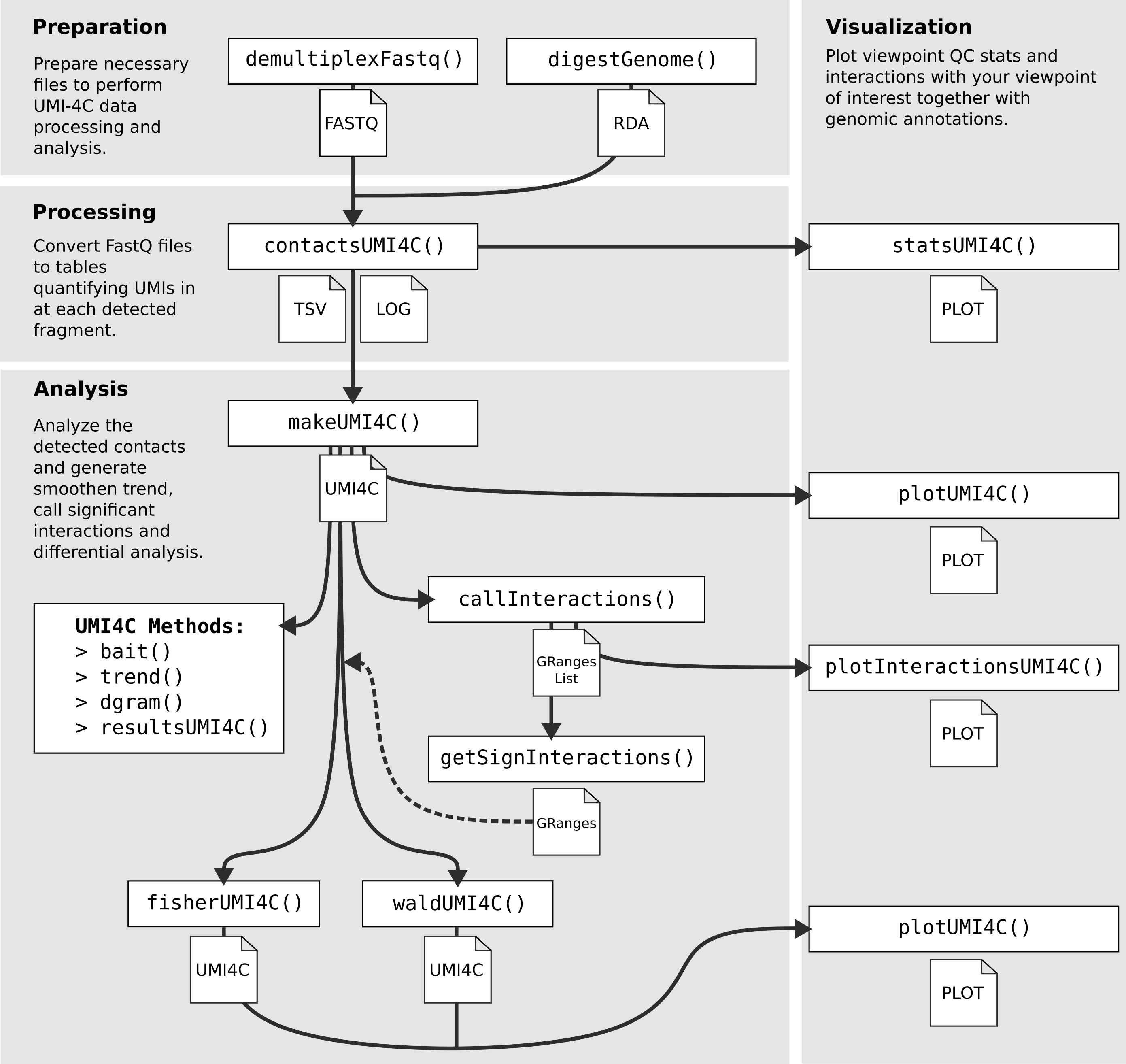
Overview of the different functions included in the UMI4Cats package to analyze UMI-4C data.
About the experimental design
One of the strengths of the UMI-4C assay (Schwartzman et al. 2016) is that of reducing the PCR duplication bias, allowing a more accurate quantification of chromatin interactions. For this reason, UMI-4C is mostly used when trying to compare changes in chromatin interactions between two conditions, cell types or developmental stages.
Taking into account this main application, UMI4Cats has been developed to facilitate the differential analysis between conditions at a given viewpoint of interest. When analyzing your data with this package, you should take into account the following points:
Each analysis (and
UMI4Cobject) should correspond to the same viewpoint. If you are analyzing different viewpoints in the same or different loci, you need to analyze them separately.The UMI4Cats package is mostly oriented to the performance of differential analysis. If you don’t have replicates yet or want to focus your analysis on a specific set of regions (like enhancers) we recommend you to use Fisher’s Exact Test (
fisherUMI4C()). If, on the other hand, you have several replicates, you can benefit from using a DESeq2 differential test specific for UMI-4C data (waltUMI4C()). You can also infer significant interactions taking advantage ofcallInteractions()andgetSignInteractions().When performing the differential analysis, UMI4Cats is only able to deal with a condition with 2 different levels. If you have more than two conditions, you should produce different UMI4C objects and perform pairwise comparisons.
About the example datasets
The datasets used in this vignette (obtained from Ramos-Rodríguez et al. (2019)) are available for download if you want to reproduce the contents of this vignette through the downloadUMI4CexampleData().
Briefly, the datasets correspond to human pancreatic islets exposed (cyt) or not (ctrl) to pro-inflammatory cytokines for 48 hours. In this example we are using the UMI-4C data generated from two different biological replicates (HI24 and HI32) using the promoter of the CIITA gene as viewpoint.
Sample datasets can be downloaded using the downloadUMI4CexampleData() function. When used without arguments, will download the full sample fastq files containing 200K reads. However, in order to reduce computing time, the Processing UMI-4C FASTQ files section in this vignette uses a reduced sample file containing 100 reads, which can be downloaded using downloadUMI4CexampleData(reduced = TRUE). The following sections addressing analysis and visualization of such data use the processed files from the 200K fastq files, which are also included inside the package and can be accessed using the system.file() function.
Quick start
In this section we summarize a complete analysis using the examples provided in this package:
## 0) Download example data -------------------------------
path <- downloadUMI4CexampleData()

## 1) Generate Digested genome ----------------------------
# The selected RE in this case is DpnII (|GATC), so the cut_pos is 0, and the res_enz "GATC".
hg19_dpnii <- digestGenome(
    cut_pos = 0,
    res_enz = "GATC",
    name_RE = "DpnII",
    ref_gen = BSgenome.Hsapiens.UCSC.hg19::BSgenome.Hsapiens.UCSC.hg19,
    out_path = file.path(tempdir(), "digested_genome/")
)

## 2) Process UMI-4C fastq files --------------------------
raw_dir <- file.path(path, "CIITA", "fastq")

contactsUMI4C(
    fastq_dir = raw_dir,
    wk_dir = file.path(path, "CIITA"),
    bait_seq = "GGACAAGCTCCCTGCAACTCA",
    bait_pad = "GGACTTGCA",
    res_enz = "GATC",
    cut_pos = 0,
    digested_genome = hg19_dpnii,
    bowtie_index = file.path(path, "ref_genome", "ucsc.hg19.chr16"),
    ref_gen = BSgenome.Hsapiens.UCSC.hg19::BSgenome.Hsapiens.UCSC.hg19,
    threads = 5
)

## 3) Get filtering and alignment stats -------------------
statsUMI4C(wk_dir = file.path(path, "CIITA"))

## 4) Analyze the results ---------------------------------
# Load sample processed file paths
files <- list.files(file.path(path, "CIITA", "count"),
                    pattern = "*_counts.tsv.gz",
                    full.names = TRUE
)

# Create colData including all relevant information
colData <- data.frame(
    sampleID = gsub("_counts.tsv.gz", "", basename(files)),
    file = files,
    stringsAsFactors = FALSE
)

library(tidyr)
colData <- colData %>%
    separate(sampleID,
        into = c("condition", "replicate", "viewpoint"),
        remove = FALSE
    )

# Make UMI-4C object including grouping by condition
umi <- makeUMI4C(
    colData = colData,
    viewpoint_name = "CIITA",
    grouping = "condition",
    bait_expansion = 2e6
)

# Plot replicates
plotUMI4C(umi, grouping=NULL)

## 5) Get significant interactions
# Generate windows
win_frags <- makeWindowFragments(umi, n_frags=8)

# Call interactions
gr <-  callInteractions(umi4c = umi,
                        design = ~condition,
                        query_regions = win_frags,
                        padj_threshold = 0.01,
                        zscore_threshold=2)

# Plot interactions
all <- plotInteractionsUMI4C(umi, gr, grouping = NULL, significant=FALSE, xlim=c(10.75e6, 11.1e6)) # Plot all regions
sign <- plotInteractionsUMI4C(umi, gr, grouping = NULL, significant=TRUE, xlim=c(10.75e6, 11.1e6)) # Plot only significantly interacting regions
cowplot::plot_grid(all, sign, ncol=2, labels=c("All", "Significant"))

# Obtain unique significant interactions
inter <- getSignInteractions(gr)

## 6) Differential testing ----------------------
# Fisher test
umi_fisher <- fisherUMI4C(umi, query_regions = iter,
                          filter_low = 20,
                          grouping="condition")
plotUMI4C(umi_fisher, ylim = c(0, 10), grouping="condition")

# DESeq2 Wald Test
umi_wald <- waldUMI4C(umi4c=umi,
                      query_regions = inter,
                      design=~condition)

plotUMI4C(umi_wald, ylim = c(0, 10), grouping="condition")
Preparing necessary files
Demultiplexing FastQ files containing multiple baits
One of the many advantages of using the UMI-4C protocol is that it allows multiplexing of different baits starting from the same sample.
To facilitate the analysis, UMI4Cats provides a function for demultiplexing the paired-end FastQ files returned by the sequencing facility: demultiplexFastq.
This function requires the following inputs:
- Name of the R1 file as input – it will automatically detect the R2.
- Barcode sequences.
- Path and name for the output files.
The barcode sequences and names to be used for each output file need to be provided as a data.frame with column names sample and barcode.
## Input files
path <- downloadUMI4CexampleData(reduced=TRUE)
fastq <- file.path(path, "CIITA", "fastq", "ctrl_hi24_CIITA_R1.fastq.gz")

## Barcode info
barcodes <- data.frame(
    sample = c("CIITA"),
    barcode = c("GGACAAGCTCCCTGCAACTCA")
)

## Output path
out_path <- tempdir()

## Demultiplex baits inside FastQ file
demultiplexFastq(
    fastq = fastq,
    barcodes = barcodes,
    out_path = out_path
)
The example FastQ file does not need demultiplexing, but the snippet above shows the steps to follow for demultiplexing a FastQ file.
Reference genome digestion
For the processing of the UMI-4C FastQ files it is necessary to construct a digested genome using the same restriction enzyme that was used in the UMI-4C experiments.
The UMI4Cats package includes the digestGenome() function to make this process easier. The function uses a BSgenome object1 as the reference genome, which is digested in silico at a given restriction enzyme cutting sequence (res_enz). Besides the restriction sequence, it is also necessary to provide, as a zero-based numeric integer, the position at which the restriction enzyme cuts (cut_pos).
In the following table you can see three examples of the different cutting sequences for DpnII, Csp6I and HindIII.
| Restriction enzyme | Restriction seq | res_enz |
cut_pos |
|---|---|---|---|
| DpnII | :GATC
|
GATC | 0 |
| Csp6I |
G:TAC
|
GTAC | 1 |
| HindIII |
A:AGCTT
|
AAGCTT | 1 |
For this example, we are using the hg19 BSGenome object and we are going to digest it using the DpnII enzyme.
library(BSgenome.Hsapiens.UCSC.hg19)
refgen <- BSgenome.Hsapiens.UCSC.hg19

hg19_dpnii <- digestGenome(
    res_enz = "GATC",
    cut_pos = 0,
    name_RE = "dpnII",
    ref_gen = refgen,
    sel_chr = "chr16", # Select bait's chr (chr16) to make example faster
    out_path = file.path(tempdir(), "digested_genome/")
)

hg19_dpnii
#> [1] "/tmp/RtmprhoiNm/digested_genome//BSgenome.Hsapiens.UCSC.hg19_dpnII"
The digested genome chromosomes will be saved in the out_path directory as RData files. The path of these files is outputted by the function, so that it can be saved as a variable (in this case hg19_dpnii) and used for downstream analyses.
Processing UMI-4C FASTQ files
Before doing any analysis, the paired-end reads stored in the FastQ files are converted to UMI counts in the digested fragments. These counts represent the contact frequencies of the viewpoint with that specific fragment. This process is implemented in the function contactsUMI4C(), which should be run in samples generated with the same experimental design (same viewpoint and restriction enzyme).
The function will consider all FastQ files in the same folder fastq_dir to be part of the same experiment (viewpoint + restriction enzyme). However, if you want to specify a subset of samples to perform the analysis you can do so by using the file_pattern argument. The R1 and R2 files for each sample need to contain _R1 or _R2 and one of the following FastQ suffixes: .fastq, .fq, .fq.gz or .fastq.gz.
For each experiment, the user needs to define 3 different sequences:
-
Bait/viewpoint sequence (
bait_seq). This is the downstream primer sequence (DS primer) that matches the sequence of the queried viewpoint. -
Padding sequence (
bait_pad). The padding sequence corresponds to the nucleotides between the DS primer end and the next restriction enzyme site. -
Restriction enzyme sequence (
res_enz). This sequence is the sequence recognized by the restriction enzyme used in the experiment.

Schematic of a UMI-4C read detailing the different elements that need to be used as input for processing the data.
Additionally, it is necessary to define the restriction enzyme cutting position (cut_pos) as previously done for the digested genome generation, together with the path of the corresponding digested genome (digested_genome) returned by the digestGenome() function.
contactsUMI4C() performs the alignment using the Rbowtie2 R package. Is thus needed to provide the corresponding reference genome indexes generated with Bowtie22. Is important to make sure that both the Bowtie2 index and the reference and digested genomes correspond to the same build (in this example, hg19).
## Use reduced example to make vignette faster
## If you want to download the full dataset, set reduced = FALSE or remove
## the reduce argument.
## The reduced example is already downloaded in the demultiplexFastq chunk.

# path <- downloadUMI4CexampleData(reduced=TRUE)
raw_dir <- file.path(path, "CIITA", "fastq")
index_path <- file.path(path, "ref_genome", "ucsc.hg19.chr16")

## Run main function to process UMI-4C contacts
contactsUMI4C(
    fastq_dir = raw_dir,
    wk_dir = file.path(path, "CIITA"),
    file_pattern = "ctrl_hi24_CIITA", # Select only one sample to reduce running time
    bait_seq = "GGACAAGCTCCCTGCAACTCA",
    bait_pad = "GGACTTGCA",
    res_enz = "GATC",
    cut_pos = 0,
    digested_genome = hg19_dpnii,
    bowtie_index = index_path,
    ref_gen = BSgenome.Hsapiens.UCSC.hg19::BSgenome.Hsapiens.UCSC.hg19,
    sel_seqname = "chr16", # Input bait chr to reduce running time
    threads = 2,
    numb_reads = 1e6 # Reduce memory usage
)
#>
#> [2021-10-28 14:23:51] Starting prepUMI4C using:
#>  > Fastq directory:
#>  /tmp/RtmprhoiNm/UMI4Cats_data_reduced/CIITA/fastq
#>  > Work directory: /tmp/RtmprhoiNm/UMI4Cats_data_reduced/CIITA
#>  > Bait sequence: GGACAAGCTCCCTGCAACTCA
#>  > Bait pad: GGACTTGCA
#>  > Restriction enzyme: GATC
#>  > Number of reads loaded into memory: 1e+06
#> [2021-10-28 14:23:52] Finished sample ctrl_hi24_CIITA
#>
#> [2021-10-28 14:23:52] Starting splitUMI4C using:
#>  > Work directory: /tmp/RtmprhoiNm/UMI4Cats_data_reduced/CIITA
#>  > Cut position: 0
#>  > Restriction enzyme: GATC
#>  > Number of reads loaded into memory: 1e+06
#> [2021-10-28 14:23:52] Finished sample ctrl_hi24_CIITA_R1.fq.gz
#> [2021-10-28 14:23:52] Finished sample ctrl_hi24_CIITA_R2.fq.gz
#>
#> [2021-10-28 14:23:52] Starting alignmentUMI4C using:
#>  > Work directory: /tmp/RtmprhoiNm/UMI4Cats_data_reduced/CIITA
#>  > Viewpoint position: chr16:10972515-10972548
#>  > Reference genome: /tmp/RtmprhoiNm/UMI4Cats_data_reduced/ref_genome/ucsc.hg19.chr16
#>  > Number of threads: 2
#> [2021-10-28 14:23:52] Finished sample ctrl_hi24_CIITA_R1.fq
#> [2021-10-28 14:23:53] Finished sample ctrl_hi24_CIITA_R2.fq
#>
#> [2021-10-28 14:23:53] Starting counterUMI4C using:
#>  > Work directory: /tmp/RtmprhoiNm/UMI4Cats_data_reduced/CIITA
#>  > Viewpoint position: chr16:10972515-10972548
#>  > Restriction enzyme: GATC
#>  > Digested genome: /tmp/RtmprhoiNm/digested_genome//BSgenome.Hsapiens.UCSC.hg19_dpnII
#> [2021-10-28 14:23:54] Finished sample ctrl_hi24_CIITA
Internally, contactsUMI4C() runs the following processes sequentially:
FastQ files preparation (
prepUMI4C). In this processing step, only reads containing thebait_seq+bait_pad+res_enzare selected. Reads with mean Phread quality scores < 20 are filtered out.Split reads at restriction sites (
splitUMI4C). Using theres_enzsequence and the cutting position (cut_pos), all R1 and R2 reads are split to mimic the fragments generated experimentally.Align split reads to the reference genome (
alignmentUMI4C).Collapse reads using UMIs (
counterUMI4C). This step is done to count real molecular events and reduce artifacts due to PCR duplicates. The function returns contacts with restriction fragments < 5Mb from the viewpoint.
Note on memory usage: For the preparation and splitting, the FastQ files are loaded into memory. If you are having problems with the memory size available in your computer, you can change the number of lines that are to be loaded using the numb_reads parameter. See ?contactsUMI4C for more information.
The final output of this process is a compressed tsv file stored in wk_dir/count, which contains the coordinates for each contact (viewpoint + contact) and the number of UMIs that support that specific interaction. These files will be used as input for the analyses performed in the following section.
Quality control measures
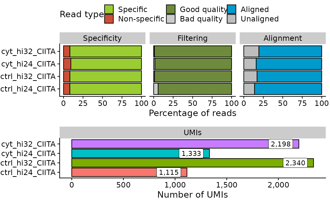
Once the processing step has been run, the statistics of the UMI-4C filtering, alignment and final number of UMIs can be generated from the logs returned by the contactsUMI4C() function. By using these logs, the function statsUMI4C() will produce a summary plot and a summary table with all statistics (wk_dir/logs/stats_summary.txt).
For demonstration purposes we used a reduced version of the fastq files to reduce comptutation time. Thus, now we will load the output of contactsUMI4C() with the full dataset, which has ben pre-computed and is saved within the UMI4Cats package.
# Using the full dataset included in the package
statsUMI4C(wk_dir = system.file("extdata", "CIITA",
    package = "UMI4Cats"
))
# Read stats table
stats <- read.delim(system.file("extdata", "CIITA", "logs", "stats_summary.txt",
    package = "UMI4Cats"
))

knitr::kable(stats)| sample_id | specific_reads | nonspecific_reads | filtered_reads | filtout_reads | al_mapped | al_unmapped | umi |
|---|---|---|---|---|---|---|---|
| ctrl_hi24_CIITA | 183831 | 16169 | 173342 | 10489 | 473730 | 75809 | 1115 |
| ctrl_hi32_CIITA | 183759 | 16241 | 181789 | 1970 | 479286 | 98065 | 2340 |
| cyt_hi24_CIITA | 181278 | 18722 | 178473 | 2805 | 479134 | 90485 | 1333 |
| cyt_hi32_CIITA | 183770 | 16230 | 182106 | 1664 | 466677 | 111822 | 2198 |
The quality control measures summarized in the plot and the table are:
-
Specific reads. Corresponds to the number of reads that contain the full viewpoint sequence (
bait_seq+bait_pad+res_enz). -
Filtered reads. Number of reads with mean Phred quality scores
>= 20. - Mapping stats. Indicates how many split reads are mapped or unmapped to the reference genome.
- UMIs. Shows the final number of molecular contacts detected.
Loading UMI-4C data into R
After processing the FastQ reads and obtaining tables summarizing number of UMIs supporting each fragment interaction with the viewpoint, the next step is to analyze such data by detecting differential contacts and visualizing the genomic interactions.
Build the UMI4C object
The first step of the UMI-4C data analysis consists in loading the tables generated by the function contactsUMI4C() and use them to construct a UMI4C object, which is based on the SummarizedExperiment class. All these steps are performed automatically by the makeUMI4C() function.
The makeUMI4C will need as input, a data frame (colData) containing all relevant experiment information that will be needed for analyzing the data later on. The mandatory columns are:
-
sampleID: Unique identifier for the sample. -
replicate: Replicate character or number identifier. -
condition: Grouping variable for performing the differential analysis. For example: “control” and “treatment,” two different cell types, etc. The condition column should only have two different values. If more condition variables are provided, the differential analysis will fail. -
file: Complete path and filename of the tsv files generated bycontactsUMI4C().
You can also include other additional columns to colData.
The UMI4C object will contain data from all the replicates. However, it might of interest group samples based on a specific variable, such as condition, to plot combined profiles or perform differential tests on merged replicates. The argument grouping controls this behavior. By default, the grouping argument is set to grouping = "condition", which will group the samples according to the variables in the condition column. These grouped UMI4C object can be accessed using groupsUMI4C(umi4c)$condition. You can also add additional groupings to a specific UMI-4C object using the addGrouping() function or avoid the calculation of grouped sample setting grouping = NULL.
Additionally, the makeUMI4C function also contains other arguments that can be used if you want to tweak the default parameters of the analysis. See ?makeUMI4C to have a complete list and description of all the arguments.
# Load sample processed file paths
files <- list.files(system.file("extdata", "CIITA", "count", package="UMI4Cats"),
                    pattern = "*_counts.tsv.gz",
                    full.names = TRUE
)

# Create colData including all relevant information
colData <- data.frame(
    sampleID = gsub("_counts.tsv.gz", "", basename(files)),
    file = files,
    stringsAsFactors = FALSE
)

library(tidyr)
colData <- colData %>%
    separate(sampleID,
        into = c("condition", "replicate", "viewpoint"),
        remove = FALSE
    )

# Load UMI-4C data and generate UMI4C object
umi <- makeUMI4C(
    colData = colData,
    viewpoint_name = "CIITA",
    grouping = "condition",
    ref_umi4c = c("condition"="ctrl"),
    bait_expansion = 2e6
)

umi
#> class: UMI4C
#> dim: 5853 4
#> metadata(7): bait scales ... ref_umi4c region
#> assays(6): umi norm_mat ... scale sd
#> rownames(5853): frag_1 frag_2 ... frag_5859 frag_5860
#> rowData names(2): id_contact position
#> colnames(4): ctrl_hi24_CIITA ctrl_hi32_CIITA cyt_hi24_CIITA
#>   cyt_hi32_CIITA
#> colData names(5): sampleID condition replicate viewpoint file
groupsUMI4C(umi)
#> List of length 1
#> names(1): condition
The makeUMI4C function will perform the following steps to generate the UMI4C object:
-
Remove fragment ends around the bait, as they are generally biased because of their proximity to the viewpoint. The value of the region that will be excluded from the analysis can be specified using the
bait_exclusionargument. The default is 3 kb. -
Focus the scope of the analysis in a specific genomic region around the bait, by default this is a 2Mb window centered on the viewpoint. The default value can be changed using the
bait_expansionargument. - Sum the UMIs of the different samples belonging to the same group (defined by the
groupingvariable). -
Obtain the normalization matrices that will be used to scale the groups to the reference, by default the group with less UMIs. If you want to avoid this normalization step, you can set
normalizedtoFALSE. - Calculate the domainograms for each group.
- Calculate the adaptive trend for each group.
Accessing UMI4C object information
The usual accessor functions from the SummarizedExperiment-class3 also work with the UMI-4C class (for example: assay, colData, etc.). Other additional accessors have been created to retrieve different information:
-
dgram(). Get a list of the domaingorams for each group. -
bait(). Retrieve a GRanges object with the bait position. -
trend(). Obtain a data.frame in long format with the adaptive smoothing trend. -
resultsUMI4C(). Retrieve results from the differential analysis. This only works if a differential analysis has been performed on the UMI4C object.
These functions can be used in the per-sample UMI4C object or in the grouped UMI4C object, which can be accessed using groupsUMI4C(umi4c)$<grouping-variable>. See an example below.
groupsUMI4C(umi) # Available grouped UMI-4C objects
#> List of length 1
#> names(1): condition

head(assay(umi)) # Retrieve raw UMIs
#>        ctrl_hi24_CIITA ctrl_hi32_CIITA cyt_hi24_CIITA cyt_hi32_CIITA
#> frag_1               0               0              0              0
#> frag_2               0               0              0              0
#> frag_3               0               2              0              0
#> frag_4               0               0              0              0
#> frag_5               0               0              0              0
#> frag_6               0               0              0              0
head(assay(groupsUMI4C(umi)$condition)) # Retrieve UMIs grouped by condition
#>        ctrl cyt
#> frag_1    0   0
#> frag_2    0   0
#> frag_3    2   0
#> frag_4    0   0
#> frag_5    0   0
#> frag_6    0   0

colData(umi) # Retrieve column information
#> DataFrame with 4 rows and 5 columns
#>                        sampleID   condition   replicate   viewpoint
#>                     <character> <character> <character> <character>
#> ctrl_hi24_CIITA ctrl_hi24_CIITA        ctrl        hi24       CIITA
#> ctrl_hi32_CIITA ctrl_hi32_CIITA        ctrl        hi32       CIITA
#> cyt_hi24_CIITA   cyt_hi24_CIITA         cyt        hi24       CIITA
#> cyt_hi32_CIITA   cyt_hi32_CIITA         cyt        hi32       CIITA
#>                                   file
#>                            <character>
#> ctrl_hi24_CIITA /__w/_temp/Library/U..
#> ctrl_hi32_CIITA /__w/_temp/Library/U..
#> cyt_hi24_CIITA  /__w/_temp/Library/U..
#> cyt_hi32_CIITA  /__w/_temp/Library/U..

rowRanges(umi) # Retrieve fragment coordinates
#> GRanges object with 5853 ranges and 2 metadata columns:
#>             seqnames            ranges strand |  id_contact    position
#>                <Rle>         <IRanges>  <Rle> | <character> <character>
#>      frag_1    chr16   9972440-9972810      * |      frag_1    upstream
#>      frag_2    chr16   9972811-9973022      * |      frag_2    upstream
#>      frag_3    chr16   9973023-9973900      * |      frag_3    upstream
#>      frag_4    chr16   9973901-9974010      * |      frag_4    upstream
#>      frag_5    chr16   9974011-9974144      * |      frag_5    upstream
#>         ...      ...               ...    ... .         ...         ...
#>   frag_5856    chr16 11970551-11971015      * |   frag_5856  downstream
#>   frag_5857    chr16 11971016-11971304      * |   frag_5857  downstream
#>   frag_5858    chr16 11971305-11971499      * |   frag_5858  downstream
#>   frag_5859    chr16 11971500-11971588      * |   frag_5859  downstream
#>   frag_5860    chr16 11971589-11972035      * |   frag_5860  downstream
#>   -------
#>   seqinfo: 1 sequence from an unspecified genome; no seqlengths

dgram(umi) # Retrieve domainograms
#> List of length 4
#> names(4): ctrl_hi24_CIITA ctrl_hi32_CIITA cyt_hi24_CIITA cyt_hi32_CIITA
dgram(groupsUMI4C(umi)$condition) # Retrieve domainograms
#> List of length 2
#> names(2): ctrl cyt

bait(umi) # Retrieve bait coordinates
#> GRanges object with 1 range and 1 metadata column:
#>       seqnames            ranges strand |        name
#>          <Rle>         <IRanges>  <Rle> | <character>
#>   [1]    chr16 10970996-10972544      * |       CIITA
#>   -------
#>   seqinfo: 1 sequence from an unspecified genome; no seqlengths

head(trend(umi)) # Retrieve adaptive smoothing trend
#>   geo_coord      trend         sd scale id_contact          sample sampleID
#> 1  10254166 0.08333333 0.03333333   150   frag_754 ctrl_hi24_CIITA     <NA>
#> 2  10254519 0.08389262 0.03355705   149   frag_755 ctrl_hi24_CIITA     <NA>
#> 3  10254871 0.08445946 0.03378378   148   frag_756 ctrl_hi24_CIITA     <NA>
#> 4  10255223 0.08503401 0.03401361   147   frag_757 ctrl_hi24_CIITA     <NA>
#> 5  10255577 0.08561644 0.03424658   146   frag_758 ctrl_hi24_CIITA     <NA>
#> 6  10255933 0.08620690 0.03448276   145   frag_759 ctrl_hi24_CIITA     <NA>
#>   replicate viewpoint file
#> 1      <NA>      <NA> <NA>
#> 2      <NA>      <NA> <NA>
#> 3      <NA>      <NA> <NA>
#> 4      <NA>      <NA> <NA>
#> 5      <NA>      <NA> <NA>
#> 6      <NA>      <NA> <NA>
Calling significant interactions
In some cases, it might be interesting to identify regions that are significantly interacting with the viewpoint. With this aim in mind, we implemented the function callInteractions(), based on the method described by Klein et al. (2015), which performs the following steps to identify significant interactions with the bait:
- Variance stabilizing transformation (VST) of the raw counts.
- Monotone smoothing modeling.
- Z-score calculation.
Of note, this method can only be applied when replicates are present for the different conditions.
Methods
4C-seq data are affected by heteroscedasticity and a signal decay from the viewpoint. These characteristics, typical of 4C-seq experiments, have to be corrected before calling statistically significant interactions with the viewpoint. To deal with heteroscedasticity in UMI4Cats, a variance stabilizing transformation (VST) is applied to the raw counts. On the other hand, signal decay is modeled using a smooth monotone function. This method is based on work by Klein et al. (2015).
Variance stabilizing transformation (VST) of the raw counts. In 4C-seq experiments, the standard deviation across samples is large for fragments with high number of contact counts. Variance stabilizing transformation (VST) is used to remove the dependence of the variance on the mean, thus correcting the dependence of the standard deviations to the contact counts abundance. This VST is performed by varianceStabilizingTransformation() from DESeq2 (Love, Huber, and Anders 2014).
Monotone smoothing modeling. The 4C-seq signal decays with genomic distance from the viewpoint and converges towards a constant level of background. 4C-seq data reflects a smooth strictly increasing or strictly decreasing function. Thus, the general decay of the 4C-seq signal with genomic distance from the viewpoint is fitted using a symmetric monotone fit. The monotone smoothing function is calculated from the transformed raw counts, using the fda package (Ramsay2005?). This function is then used to generate the fitted count values.
Once the counts are VST transformed and the signal decay is fitted using a symmetric monotone fit, the z-scores are inferred to identify statistically significant interactions with the viewpoint.
Z-score calculation. Z-scores are calculated dividing the residuals values obtained from the VST-normalized and fitted counts, by the median absolute deviation (MAD) of all the sample’s residuals. Z-scores are then converted into one-sided p-values using the standard normal cumulative distribution function. Finally, a false discovery rate (FDR) multiple testing correction is performed to reduce type I error. Regions significantly interacting with the viewpoint can then be defined as those fragments with a significant adjusted p-values and passing the z-score threshold.
Obtaining significant interactions
To identify significant interactions, the user needs to provide a set of regions that will be used to calculate the z-scores. These regions can be enhancers, open chromatin regions, a list of putative regulatory elements in the locus or, when no candidate regions are available, the user can take advantage of the makeWindowFragments() function to join a fixed number of restriction fragments into windows.
Next, these candidate regions (query_regions) and the UMI4C object need to be provided to the callInteractions() function. The function will return a GRangesList with each element corresponding to the specific z-scores and significance status of the query_regions in a specific sample. This information can be visualized by using the plotInteractionsUMI4C() function.
Finally, the function getSignInteractions() can be used to obtain a GRanges object with the regions that were found to be significant in at least one of the samples. This output can be used later to guide the identification of differential interactions.
# Generate windows
win_frags <- makeWindowFragments(umi, n_frags=8)

# Call interactions
gr <-  callInteractions(umi4c = umi,
                        design = ~condition,
                        query_regions = win_frags,
                        padj_threshold = 0.01,
                        zscore_threshold=2)

# Plot interactions
all <- plotInteractionsUMI4C(umi, gr, grouping = NULL, significant=FALSE, xlim=c(10.75e6, 11.1e6)) # Plot all regions
sign <- plotInteractionsUMI4C(umi, gr, grouping = NULL, significant=TRUE, xlim=c(10.75e6, 11.1e6)) # Plot only significantly interacting regions
cowplot::plot_grid(all, sign, ncol=2, labels=c("All", "Significant"))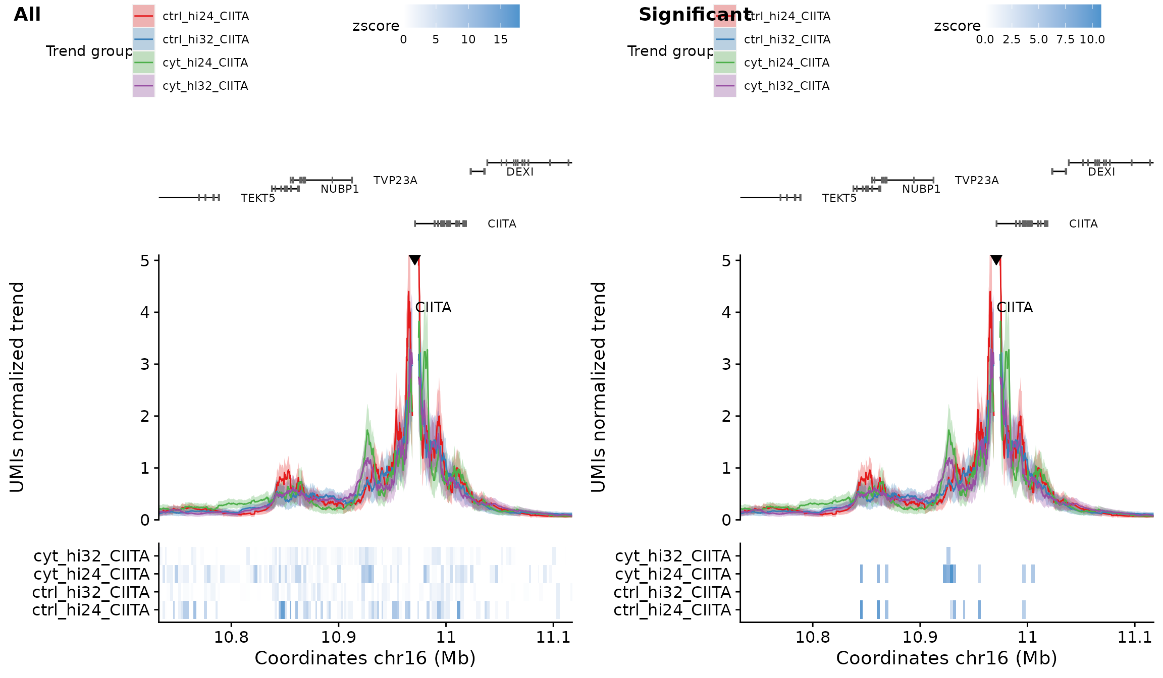
# Obtain unique significant interactions
inter <- getSignInteractions(gr)
#>
#>  Results
#>
#> Iter.   PENSSE   Grad Length Intercept   Slope
#> 0        0.2265      0.0136      3.5982      -0.3584
#> 1        0.2071      0.0149      4.869      -0.5465
#> 2        0.2017      0.0059      5.3134      -0.6115
#> 3        0.2005      0.0035      5.5585      -0.6523
#> 4        0.2002      0.0017      5.6902      -0.674
#>
#>  Results
#>
#> Iter.   PENSSE   Grad Length Intercept   Slope
#> 0        0.1368      0.0173      4.046      -0.4279
#> 1        0.1211      0.0126      4.8615      -0.5634
#> 2        0.1142      0.0077      5.4498      -0.651
#> 3        0.1124      0.0032      5.6524      -0.6863
#> 4        0.112      0.0021      5.8503      -0.7202
#>
#>  Results
#>
#> Iter.   PENSSE   Grad Length Intercept   Slope
#> 0        0.2366      0.0162      3.831      -0.3946
#> 1        0.2156      0.0138      4.9162      -0.5662
#> 2        0.2071      0.0067      5.5897      -0.6631
#> 3        0.205      0.0034      5.8431      -0.7058
#> 4        0.2044      0.0016      6.0693      -0.7434
#> 5        0.2043      6e-04      6.1188      -0.7519
#>
#>  Results
#>
#> Iter.   PENSSE   Grad Length Intercept   Slope
#> 0        0.1589      0.0161      4.0274      -0.4237
#> 1        0.1465      0.0102      4.6641      -0.5325
#> 2        0.1407      0.0063      5.213      -0.6163
#> 3        0.1392      0.0026      5.3826      -0.6463
#> 4        0.1387      0.0014      5.5676      -0.6785
Differential analysis
Once the UMI4C object is generated, you can perform a differential analysis between conditions using two different approaches. In both cases you can provide query_regions, such as enhancers, open chromatin regions or the output getSignInteractions() to focus the analysis in regions that are more likely to have differential interactions.
DESeq2’s Wald Test (
waldUMI4C()). We recommend using this test to detect significant differences, as it performs a more sophisticated modeling and testing of count data (Love, Huber, and Anders 2014). To obtain reliable results we recommend using several replicates with a high number of UMIs per sample.Fisher’s Exact Test (
fisherUMI4C()). In some instances, having insufficient replicates or UMI depth precludes the use of dESeq2’s Wald Test. In such cases, the user can opt for the Fisher’s Exact Test, which can provide useful results when used in a set of candidate regions, such as enhancers or the output ofcallInteractions().
Differential Analysis using DESeq2
The funciton waldUMI4C() performs a differential analysis using the DESeq() function from the DESeq2 package. For specific details on the algorithm please see Love, Huber, and Anders (2014), the DESeq2 vignette or ?DESeq2::DESeq.
umi_wald <- waldUMI4C(umi,
                      query_regions = inter,
                      design = ~condition)
#> converting counts to integer mode
#> estimating size factors
#> estimating dispersions
#> gene-wise dispersion estimates
#> mean-dispersion relationship
#> -- note: fitType='parametric', but the dispersion trend was not well captured by the
#>    function: y = a/x + b, and a local regression fit was automatically substituted.
#>    specify fitType='local' or 'mean' to avoid this message next time.
#> final dispersion estimates
#> fitting model and testing
Differential analysis using Fisher’s Exact Test
To perform Fisher’s EXact test, queried regions (query_regions) will be first filtered according to the number of UMIs present in the filter_low parameter. You can reduce this number or disable filtering using filter_low = FALSE.
Then, a contingency table for each region where the differential test should be performed will be created, where the group stored in metadata(umi)$ref_umi4c will be used as references. The values on the contingency table correspond to the following:
| Group | Query region | Region |
|---|---|---|
| Reference | \(n1\) | \(N1 - n1\) |
| Condition | \(n2\) | \(N2 - n2\) |
Where \(N1\) and \(N2\) correspond to the total number of UMIs in the whole analyzed region (metadata(umi)$region) and \(n1\) and \(n2\) correspond to the total number of UMIs in the query region that is to be tested.
After all the Fisher’s Exact Tests are performed, p-values are adjusted using the FDR method. Query regions with adjusted p-values > 0.05 will be considered significantly different. Check ?fisherUMI4() for more information and additional arguments you can provide to the function.
# Perform differential test
umi_fisher <- fisherUMI4C(umi,
                          grouping = "condition",
                          query_regions = inter,
                          filter_low = 20)
Retrieve differential analysis results
Results from both Fisher’s Exact test and DESeq2 can be retrieved using the resultsUMI4C() on the UMI4C object returned by both functions.
resultsUMI4C(umi_fisher, ordered = TRUE, counts = TRUE, format = "data.frame")
#>    seqnames    start      end        id mcols.position umis_ref umis_cond
#> 21    chr16 10924799 10927966 region_21       upstream       12        46
#> 9     chr16 10927967 10930640  region_9       upstream       13        41
#> 22    chr16 11003893 11006616 region_22     downstream       18        35
#> 13    chr16 10995350 10998148 region_13     downstream       40        26
#> 11    chr16 10940371 10941822 region_11       upstream       31        22
#> 10    chr16 10930641 10933175 region_10       upstream       25        34
#> 12    chr16 10954198 10956424 region_12       upstream       49        43
#> 20    chr16 10921487 10924798 region_20       upstream       30        34
#> 1     chr16 10299502 10301622  region_1       upstream        8         7
#> 2     chr16 10310432 10313385  region_2       upstream        9         2
#> 3     chr16 10353878 10356964  region_3       upstream        5         9
#> 4     chr16 10600203 10602402  region_4       upstream        2        10
#> 5     chr16 10607341 10610133  region_5       upstream       10         6
#> 6     chr16 10844428 10846299  region_6       upstream       12        26
#> 7     chr16 10860016 10862414  region_7       upstream       13        26
#> 8     chr16 10867157 10870182  region_8       upstream       19        14
#> 14    chr16 11359876 11364163 region_14     downstream        8        10
#> 15    chr16 11388250 11390925 region_15     downstream        9         2
#> 16    chr16 11454752 11456873 region_16     downstream       10         2
#> 17    chr16 11523568 11525795 region_17     downstream        8         0
#> 18    chr16 10625425 10629517 region_18       upstream        7        19
#> 19    chr16 10638100 10640012 region_19       upstream        1        12
#>          pvalue odds_ratio log2_odds_ratio         padj  sign
#> 21 8.147506e-06  3.7803109       1.9185049 6.518005e-05  TRUE
#> 9  1.741669e-04  3.1045960       1.6344056 6.966677e-04  TRUE
#> 22 2.695884e-02  1.9070663       0.9313550 7.189023e-02 FALSE
#> 13 8.243309e-02  0.6310408      -0.6641949 1.648662e-01 FALSE
#> 11 2.144470e-01  0.6901586      -0.5350001 3.431152e-01 FALSE
#> 10 2.974309e-01  1.3303588       0.4118154 3.965746e-01 FALSE
#> 12 4.640309e-01  0.8540839      -0.2275503 5.303210e-01 FALSE
#> 20 7.078802e-01  1.1067929       0.1463853 7.078802e-01 FALSE
#> 1            NA         NA              NA           NA    NA
#> 2            NA         NA              NA           NA    NA
#> 3            NA         NA              NA           NA    NA
#> 4            NA         NA              NA           NA    NA
#> 5            NA         NA              NA           NA    NA
#> 6            NA         NA              NA           NA    NA
#> 7            NA         NA              NA           NA    NA
#> 8            NA         NA              NA           NA    NA
#> 14           NA         NA              NA           NA    NA
#> 15           NA         NA              NA           NA    NA
#> 16           NA         NA              NA           NA    NA
#> 17           NA         NA              NA           NA    NA
#> 18           NA         NA              NA           NA    NA
#> 19           NA         NA              NA           NA    NA
The parameter counts indicates whether raw counts used for the test should be outputted. In Fisher’s Exact Test, umis_ref corresponds to the number of raw UMIs from the sample/group used as reference (accessible through metadata(umi_dif)$ref_umi4c).
Visualizing UMI-4C contact data
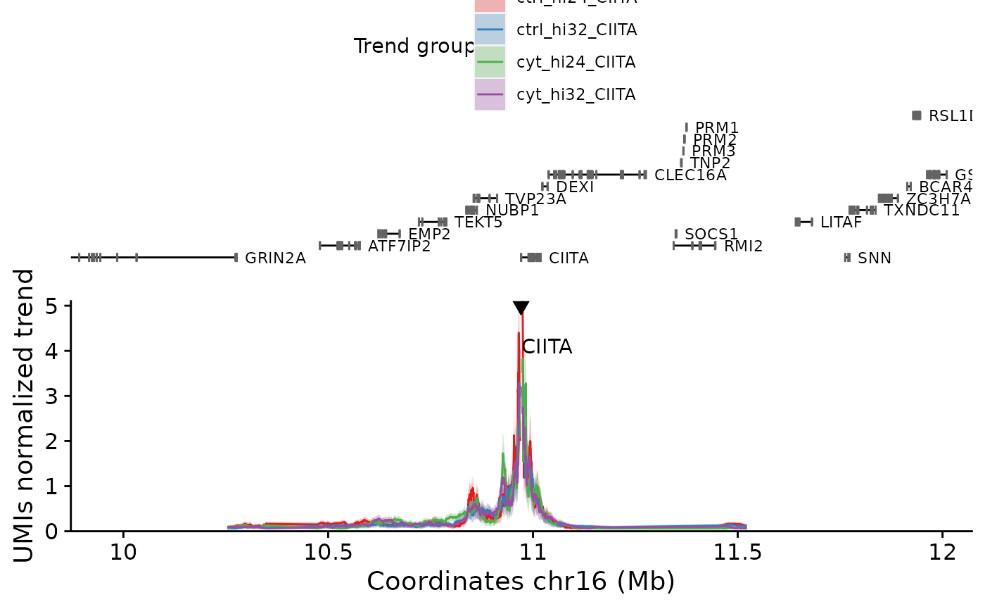
Once the UMI4C object is created, you can visualize detected chromatin interactions using the plotUMI4C function.
The gene annotations will be extracted from the TxDb.Hsapiens.UCSC.hg19.knownGene package by default. Make sure that the annotations coincide with your reference genome. You can check the package GenomicFeatures for more information on available TxDb objects. The domainogram plotting is controlled by the dgram_plot argument. If you set it to FALSE, the domainogram will not be plotted.
In case you are interested in plotting the profiles of the different samples contained in your experiment, you just need to set the grouping argument to NULL, which will disable sample grouping:
plotUMI4C(umi,
    grouping = NULL,
    TxDb = TxDb.Hsapiens.UCSC.hg19.knownGene::TxDb.Hsapiens.UCSC.hg19.knownGene,
    dgram_plot = FALSE
)
If the UMI4C object contains information on the differential contacts, this data will be shown in the plot as well. The grouping argument uses the grouped trends and domainograms stored in groupsuMI4C(). If you want to add a new grouping, you can use the addGRouping() function.
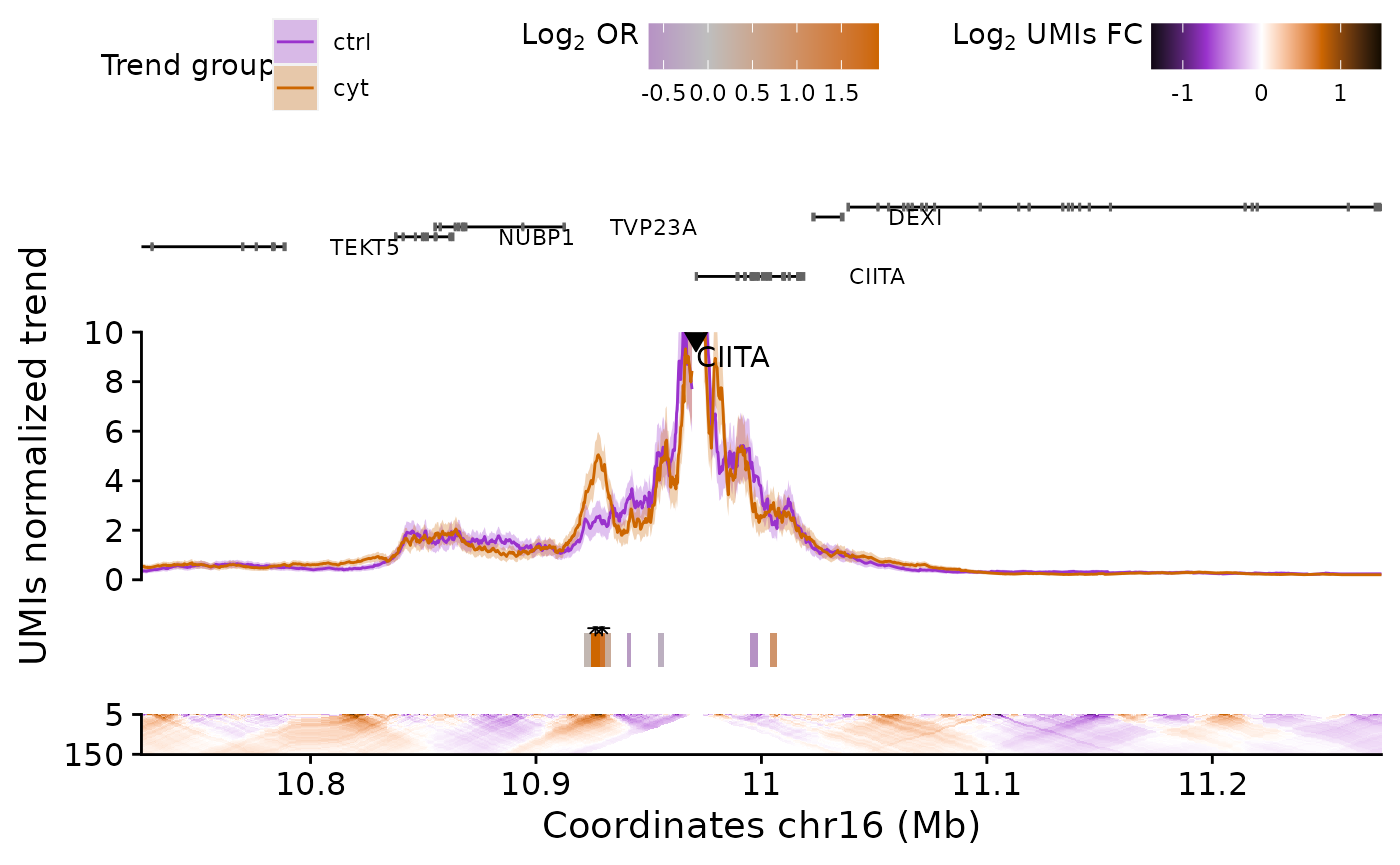
There are several different arguments you can provide to plotUMI4C to modify the output plot. You can check them by typing ?plotUMI4C in your R console.
The plotUMI4C function is a wrapper for separate functions that plot the different elements included in the figure. You can use each of the functions separately if you are interesting in combining them differently or with other ggplot2 objects. Check each function documentation at ?plotTrend, ?plotGenes, ?plotDomainogram and ?plotDifferential.